Assignment 6

Goals: The goals of this assignment is to gain knowledge in SPSS in relation to regression analysis and be able manipulate data in Excel as well as map standardized residuals in ArcGIS.

Part 1:

Introduction:
Crime and poverty is always at a topic of interest for many policy makers. A particular town was included in a study on crime rates and poverty. The towns news station stated that crime increases as the number of kids who get free lunches increases, according to a particular data source. This is a strong claim from the news station, which deserves a further glance at the data. To see if this claim is correct, SPSS will be used to complete a regression to observe whether there actually is a relationship between the number of kids who receive free lunch and crime rates.

Methods:
To determine whether there is relationship between the independent variable (free lunches) and the dependent variable (crime rates), the data provided in an Excel document was used to create a scatter plot and OLS line (Figure 1). After that, the same data was uploaded into SPSS and a linear regression analysis was used to show the linear relationship between each variable (Figure 2). This analysis is important because it displays the regression coefficient (b) that explains how responsive the dependent variable is to change in the independent variable. More simplistically, it gives the direction of the relationship between each variable. Additionally, the analysis provides the coefficient of determination ( r²) which represents how the independent variable explains the dependent variable.

Figure 1: Scatter Plot Between Independent and Dependent Variables 

Figure 2: Linear Regression Analysis

Results:

By looking at the scatter plot and trend line, it is clear there is a somewhat positive relationship between the percentage of kids getting free lunch and crime rates. This relationships can be confirmed by looking at the regression coefficient (0.173) which shows the positive slope. Because .173 is significantly closer to 0 that it is to 1, this means that the relationship between the two variables is weak. It is also important to pay attention to the significance level: 0.005 (two-tailed test). This means that in relation to the hypothesis test of this analysis, the null hypothesis would be rejected because there is a relationship between the independent and dependent variables. If a new area of town turned out to have 30% of the kids having free lunch, the crime rate would then be 72.38. To determine this result the trend line equation was used: y=1.6852x+21.819 with 30 going in as 'x'. Although these variables show an existing relationship, it wouldn't be best to base assumptions off of these results due to the weak regression coefficient. 

Conclusion:

According to the results from the scatter plot and the linear regression analysis, the local news station was correct in saying that there was a positive relationship between the percentage of kids that receive free lunch and crime rates. However, the relationship between both variables is very weak which means that there might be other factors that effect each of these variables more than each other. To tie these variables together without knowing the cause would be misleading. Correlation does not imply causation. This variables should be examined individually before the news station shares this information with the town. 

Part 2:

Introduction: 

The city of Portland, Oregon is worried about whether the responses to 911 calls are sufficient. For better understanding, different factors will be looked at to help determine what areas most of the calls are coming from. This information will be useful to a company that wants to construct a new hospital so they can know where to place the ER and how big to build it. By analyzing which areas most of the 911 calls are coming from, the most accurate area of placement can be determined for the proposed hospital. 

Methods:

To start, data featuring number of 911 calls per census tract, number of people with no high school degree, number of people unemployed, and the number of people who were foreign born were created into three different scatter plots in Excel (Figure 3,4,5,6,7,8). The number of calls always being the dependent variable, and the other three variables representing the independent variables. Next, using SPSS, using calls as the dependent variable again and the other three as independent variables, a linear regression analysis was performed for each of the three combinations of data. After that, ArcGIS was used to create a choropleth map to show the number of 911 calls per Census Tract (Figure 9). Also, an additional standardized residual map was created to display the variable with the largest r² value (Figure 10). This map essentially shows the standard deviation of the residuals or the amount of deviation from the regression line. All of this information will aid in testing the hypothesis. The null hypothesis: there is no linear relationship between the number of 911 calls and the number of people with no high school degree, number of people unemployed, and the foreign born population. The alternative hypothesis: there is a linear relationship between the number of  911 calls and the number of people with no high school degree, number of people unemployed, and the foreign born population                

Results:

Figure 3: Low Education and 911 Calls Graph

Figure 4: Low Education and 911 Calls Analysis

Looking at Figure 3 & 4, there is a positive slope represented from the trend line. The regression coefficient of 0.567 also shows positive slope and a fair strength between the variables. The significance level is at 0.000 meaning that there is a significant linear relationship between 911 calls and the number of people with no high school degree. This means that we can reject the null hypothesis. The equation y=0.166x+3.931 tells us that every person without a high school degree,  means that there is a 0.166 increase of 911 calls. 

Figure 5: Unemployment and 911 Calls Graph

Figure 6: Unemployment and 911 Calls Analysis

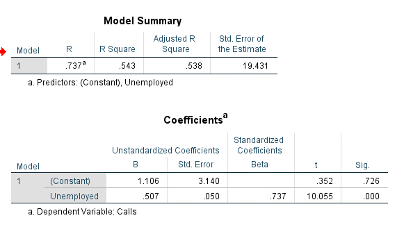
Looking at Figure 5 & 6, there is a positive slope represented from the trend line. The regression coefficient of 0.543 also shows a positive slope and a fair strength between the variables. The significance level is once again at 0.000 meaning there is a significant linear relationship between 911 calls and the number of people who are unemployed. This means that we can reject the null hypothesis. The equation y=0.507x+1.106 tells us that each person who is unemployed, increases the number of 911 calls by 0.507. 

Figure 7: Foreign Born Population and 911 Calls Graph

Figure 8: Foreign Born Populations and 911 Calls Analysis

Looking at Figure 7 & 8, there is a positive slope represented from the trend line. The regression coefficient of 0.552 also shows a positive slope and a fair strength between the variables. The significance level is once again at 0.000 meaning there is a significant linear relationship between 911 calls and the number of people who were foreign born. This means that we can reject the null hypothesis. The equation y=0.080x+3.043 tells us that each person who was foreign born, increases the number of 911 calls by 0.080. 

Figure 9: Choropleth Map

Figure 10: Standardized Residual Map

Figure 9 displays the choropleth map of the number of 911 calls per census tract in Portland, OR. The darkest blue tracts represent the highest numbers of 911 calls and then ranges down to the lightest blue representing very few calls. It looks like the most calls are coming from the census tracts located in the upper middle of Portland. The independent variable that had the highest  r² value turned out to be number of people with no high school degree. Figure 10 shows data that represents the number of 911 calls and the the number of people with no high school degree per census tract. Standard deviation helps to show which census tracts fell above or below the regression line. Red meaning above and blue meaning below. This means that these areas have higher or lower calls than the regression line predicted. When comparing Figure 9 and Figure 10, the two dark red census tracts on Figure 10 are also shown as dark blue on Figure. This makes sense considering both maps show significant number of 911 calls coming from those census tracts. 

Conclusion: 

On Figure 10, two census tracts are highlighted in between two other census tracts that were over 2.5 standard deviations. The two highlighted tracts were chosen because they are directly located between the two census tracts with high 911 calls. This would a good area for a potential hospital. Although it would be located in an area that doesn't have the highest calls, it would directly between two areas that do have high calls so that the people in need of an ER will be equally close respectively from both sides. Although the independent variable that had the highest  r² value turned out to be number of people with no high school degree, the other two variables had very similar r² values as well and should also be considered when examining locations to put potential hospitals. 

Assignment 5

Introduction: 
The purpose of this assignment was to learn how to analyze correlation and spatial autocorrelation while using Excel, SPSS and GeoDa. This assignment is separated into two sections and each part uses different data and requires critical thinking skills to understand the correlations and explain the patterns.

Part 1: Correlation
Question1:
For part one of this assignment, a scatter plot was created and a trend line was inserted in Excel from information provided relating to the correlation between distance (ft) and sound level (dB)(Figure 1).

Figure 1: Scatter Plot

Next, SPSS was created to make a bivariate correlation to find the Pearson Correlation (Figure 2).

Figure 2: Pearson Correlation

Now with all of the necessary information, the hypothesis can be determined. So, the null hypothesis is that there is no correlation between the distance (ft) and sound level (dB). The alternative hypothesis states that there is a correlation between the distance (ft) and sound level (dB). By looking at the results from the Pearson Correlation at -.896, it is observed that there is a negative correlation between the variables. It is a strong negative relationship between sound level and distance because the Pearson Correlation was so close to -1. Also, the significant level ended up being 0.000 which is smaller than 0.005, so we can reject the null hypothesis because there is clearly a correlation between distance and sound level.

Question 2: 
After that, a correlation matrix was created in SPSS using data from census tracts and population in Detroit, Michigan (Figure 3). This data holds information about different races in Detroit as well as other variables like Finance, Bachelor's Degrees, Median Household Income, etc. The correlation matrix shows relationships between each of these variables.

Figure: 3: Correlation Matrix

By looking at the matrix correlation we can observe a few patterns. First of all, there is a positive relationship between the White population and having a bachelor's degree. This significance level for the two tailed test is at 0.000 marked by two asterisks indicating this correlation is significant at the 0.01 level.  Black and Asian populations also showed a correlation with having a bachelor's degrees but just not as high as White populations. The Hispanic population is the only one that doesn't have a correlation. Also, there is correlation between the Black and Asian populations with the manufacturing industry. The significance is at the 0.01 level for Black populations and the 0.05 level for the Asian populations. The correlations for the White and Hispanic populations are not significant for the manufacturing industry. Another notable pattern is between the retail industry and the White, Back, and Asian populations. White and Asian both have positive correlations while Black populations have a negative correlation. It appears that once again the Hispanic populations don't have a significant correlation with this category; this seems to be the trend amongst the other variables as well. A few assumptions I could make with the results of this correlation matrix is that the White and Asian populations seem to have a positive correlation with almost all of the variables listed. Black populations on the other hand seem to have negative correlations with each of the variables.

Part 2: Spatial Autocorrelation

Introduction:
For the second part of this assignment, I have been asked by the Texas Election Commission (TEC)  to analyze the patterns from the presidential elections from the years 1980 and 2012. The TEC has provided data from those election years in hopes that observations can be made about different patterns so they can inform the governor of Texas whether or not the voting patterns have changed between the 32 years. The specific data provided that has been given from the TEC is voter turnout and the percent Democratic vote for both election years. The information I will need to retrieve myself is the percent Hispanic populations for 2010 as well as the Texas state shapefile from the US census.

Methods:
To start, the percent Hispanic populations for 2010 in Texas from the US Census website was downloaded. The data included a lot of other unneeded variables so there needed to be a reduction from the amount of columns from the excel file to just the percent Hispanic. Next, the Texas shapefile was downloaded from the US Census website as well. After all of the data components were collected, ArcMap was opened and then uploaded the Texas shapefile and joined the percent Hispanic data and the data provided by the TEC through the Geo_ID field. After all the table were joined, I exported the new combined data as a shapfile so I could then open it in GeoDa and start to analyze the relationships between percent Hispanic populations, voter turnout, and the percent Democratic vote to determine whether there is a spatial autocorrelation between them. Once my new Texas shapefile was uploaded into GeoDa, I created a spatial weight with rook continuity. Then, scatter plots representing the Moran's I were created for voter turnouts and the percent Democratic vote for the years 1980 and 2012 as well as the percent Hispanic population for 2010 (5 scatter plots total). Also, LISA cluster maps were created for each of the five variables as well.

Results:
***Before displaying the map results, some background information about what the LISA cluster maps are showing is needed first. The red shown on the maps represents areas of High-High (+,+), which means that a specific area of high value is surrounded by other areas of high value. The pink shown on the maps represents areas of High-Low (+,-) which means that an area of high value is surrounded by low values and is considered an outlier. The blue shown on the maps represents areas of Low-Low (-,-), which means that an area of low value is surrounded by other areas of low value. Lastly, the light blue shown on the maps represents areas of Low-High (-,+), which means that an area of low value is surrounded by areas of high value and is also considered an outlier. Any white value indicates no significance. This information is important to know when analyzing LISA maps.

1980 Voter Turnout: The scatter plot (Figure 4) and the LISA map (Figure 5) really helps represent the data visually. The scatter plot shows a slight positive correlation with a Moran's I of 0.468. The LISA map shows high voter turnouts in northern Texas as well as a small area in the center. Low voter turnout ares are in southern and eastern Texas.

Figure 4: Scatter Plot of Voter Turnout in1980

Figure 5: LISA Map of Voter Turnout in 1980

2012 Voter Turnout: The scatter plot (Figure 6) for voter turnout in 2012 also has a very slight positive correlation with a Moran's I of 0.336. The LISA map (Figure 7) once again shows a low voter turnout for southern Texas. However, the year 2012 didn't have as many areas with high voter turnout.

Figure 6: Scatter Plot of Voter Turnout in 2012

Figure 7: LISA Map of Voter Turnout in 2012

1980 Percent Democratic Vote: The scatter plot (Figure 8) for the percent Democratic vote in 1890 has a more significant positive correlation than the others so far and has a Moran's I of 0.575. The LISA map (Figure 9) shows a low percent of Democratic voters in the northern part of the panhandle of Texas. There is a high percentage of Democratic voters in the southern tip of Texas as well as some of the eastern side.

Figure 8: Scatter Plot of Percent Democratic Voters 1980

Figure 9: LISA Map of Percent Democratic Voters 1980

2012 Percent Democratic Vote: The scatter plot (Figure 10) for the percent Democratic vote in 2012 shows another strong positive correlation along with a Moran's I of 0.696. The LISA map (Figure 11) shows some interesting differences between percent Democratic vote in 2012 compared to 1980. It looks like there were more counties with a low percent of Democratic this time around. Also, high areas of Democratic voters were now located in counties on the western side of the state instead of the eastern side. 

Figure 10: Scatter Plot of Percent Democratic Voters 2012

Figure 11: LISA Map of Percent Democratic Voters 2012

Percent Hispanic Population: The scatter plot (Figure 12) for the percent Hispanic populations additionally shows a high positive correlation with a Moran's I of 0.779. The LISA map (Figure 13) for percent Hispanic populations shows counties with low percents in the northeastern part of the state and counties with high percents in the southwestern part of the state. This LISA map also showed the least amount of outliers of all five.

Figure 12: Scatter Plot of Percent Hispanic Populations 

Figure 13: LISA Map of Percent Hispanic Populations

Conclusion:
Scatter plots and LISA maps are great ways to represent and visualize different sets of data so it is easier to find autocorrelations. A few correlations are discovered from these maps. First of all, high percents of democratic voters tend to be counties that also have high percents of Hispanic populations. This makes sense due to the fact that most Hispanic populations do tend to vote democratic. An interest difference that related back to the study question is that there were less counties with high voter turnout in 2012 compared to 1980. This could have been influenced by who was running for president at the time. Another interesting observation was the locational transition of voters from the percent Democratic populations in 1980 to 2012. There was a high percent of Democratic voter turnout on the eastern side of Texas in the 1980 election but in the 2012 election those some counties became insignificant and counties across the state on the western side became high percent. The cause of that transition would be of interest to look into further. Another notable observation is from Figure 13. This LISA map shows the smallest amount of outliers but those counties are located in interesting areas where there must be a significant reason for that outcome. Overall, the TEC could inform the governor of Texas that there have been a decrease of voter turnout since 1980 and that counties that have high percents of Hispanic populations will most likely have high percents of Democratic voter turnout.

Assignment 4

Introduction: 
For the objective of this assignment, I will learn how to calculate 'z' and 't' tests as well as know when to use them for different situations. This will also involve using the steps of hypothesis testing which is very important for the scientific method. From the hypothesis test, I will be able to make decisions about the null and alternative hypothesis along with actually utilizing real world data to connect the statistics and geography. 

Key Terms:
I will first define and explain some key terms that will help with the  better understanding of hypothesis tests.

Null Hypothesis: When performing a hypothesis test, the goal is to see whether the hypothesized mean is the same or different than the observed mean. The null hypothesis says that there is no difference between the observed mean and they hypothesized mean (or equals 0).

Alternative Hypothesis: The alternative hypothesis states that yes, there is a difference between the hypothesized mean and the observed mean (or equals 0). 

Reject or Fail to Reject: When performing a hypothesis test, the question we are trying to ask is whether we reject or fail to reject the null hypothesis, we never just accept it. By rejecting the null hypothesis, we are saying that there is a difference between the means. When we say fail to reject, we are are acknowledging that there are no differences between the mean. 

Steps in Hypothesis Testing:
1. State the null hypothesis 
2. State the alternative hypothesis
3. Choose a statistical test
4. Choose α or the level of significance
5. Calculate test statistic 
6. Make decision about the null and alternative hypothesis 

Part One: 

Question 1: For part one of the assignment, I was given a chart that was partially filled with information about 't' and 'z' tests. My responsibility was to complete the rest of the chart (Figure 1) filling in the spaces of 'α' which is the significance level for the test, 'z or t' which is asking for t-test or z-test, and 'z or t value' which is asking for the critical value for the significance level. 

Figure 1: Chart containing information on 'z' and 't' tests.

Question 2: For the second question, we were given the following scenario:
In Kenya, the Live Stock Development Organization and the Department of Agriculture estimate that yields in a certain district should approach the following amounts in metric tons (averages based on  data from the whole country) per hectare: groundnuts. 0.55; cassava, 3.8; and beans, 0.28. Data was collected from 23 farmers that conclude to these results: 

           μ          σ

Ground Nuts  0.51 0.3

        Cassava   3.4            .74

     Beans  0.33      0.13

With the given information, I will now be able to test the hypothesis for each of these products. For

these tests, I will be able to assume that they are two-tailed tests with a Confidence Level of 95%. I will also be determining the probability of each crop and explaining the differences in my results. The statistical test I chose was a T-test because the sample size (n) is under 30. 

Ground Nuts

1. Null Hypothesis: There is no difference between the yield of ground nuts from the sample farmers compared to the county as a whole. 
2. Alternative Hypothesis: There is a difference between the yield of ground nuts from the sample farmers compared to the county as a whole. 
3. T-test
4. Level of Significance: 95%, Two Tailed 0.025
5. Calculation (Figure 2): -0.64

6. This is a two tailed test with a significance of 95% and critical values of -2.07 to 2.07. So, because -0.64 falls between -2.07 and 2.07, we fail to reject the null hypothesis. This means that there is not a difference between the yield of ground nuts from the sample farmers compared to the county as a whole. 
Probability: 26.4%

Figure 2: Test calculation for ground nuts.

Cassava:
1. Null Hypothesis: There is no difference between the yield of cassava from the sample farmers compared to the county as a whole. 
2. Alternative Hypothesis: There is a difference between the yield of cassava from the sample farmers compared to the county as a whole.
3. T-test
4. Level of Significance: 95%, Two Tailed 0.025
5. Calculation (Figure 3): -2.59
6: Because the significance is the same, the critical values are still the same at + or -2.07. So, because -2.59 does not fall between -2.07 and 2.07, we reject the null hypothesis. This means that there is a difference between the yield of cassava from the sample farmers compared to the county as a whole. 
Probability: 0.84%

Figure3: Test calculation for cassava. 

Beans:
1. Null Hypothesis: There is no difference between the yield of beans from the sample farmers compared to the county as a whole.
2. Alternative Hypothesis: There is a difference between the yield of beans from the sample farmers compared to the county as a whole.
3. T-test
4. Level of Significance: 95%, Two Tailed 0.025
5. Calculation (Figure 4): 1.84
6. Because the significance is the same, the probability is still the same at + or -2.07. So, because 1.84 falls between -2.07 and 2.07, we fail to reject the null hypothesis. This means that there is not a difference between the yield of beans from the sample farmers compared to the county as a whole.
Probability: 96.03%

Figure 4: Test calculation for beans.

Similarities and Differences: Both ground nuts and beans failed to reject the null hypothesis which shows that there was not a difference between the yield of that product from the sample farmers compared to the county as a whole. However, Cassava actually rejected the hypothesis. Cassava is the only product that showed a difference between the yield of the sample farmers compared to the county as a whole.

Question 3: I have now been asked to look at whether the level of pollutants in a stream is over the allowable limit of 4.4 mg/l. The sample size (n) is 17 with the mean pollutant level at 6.8mg/l and a standard deviation of 4.2. This test will also have a significant level of 95% but with as one tailed test.

Level of Pollutants:
1. Null Hypothesis: There is no difference between the sample mean pollutant level of 6.8 and the allowable limit of 4.4.
2. Alternative Hypothesis. There is a difference between the sample mean pollutant level of 6.8 and the allowable limit of 4.4.
3. T-test: n is under 30
4. Level of Significance: 95%, One Tailed 0.05
5. Calculation (Figure 5): 2.36

6. This is a one tailed test with a significance of 95% and a critical value of 1.75. The result was 2.36 which is higher than 1.75. This means that we reject the null hypothesis and that there is a difference between the sample mean pollutant level of 6.8 and the allowable limit of 4.4. This proves that the pollutant levels are higher than the allowable limit.
Probability: 98.6%

Figure 5: Test calculation for level of pollutants. 

Part Two:
For part two of the assignment, I have created a map (Figure 6) displaying the average value of homes per county block in Eau Claire county. My objective was to see whether the the average value of homes for the City of Eau Claire block groups are significantly different from the block groups for Eau Claire County. I will be using at Z-test to determine this because the sample size (n) is greater than 30. 

Average Value of Homes:
1. Null Hypothesis: There is no difference between the average values of homes in the city of Eau Claire compared to the county of Eau Claire. 
2. Alternative Hypothesis: There is a difference between the average values of homes in the city of Eau Claire compared to the county of Eau Claire.
3. Z-Test: n is over 30.
4. Level of Significance: 95%, Two Tailed 0.025
5. Calculation (Figure 7): -2.57
6. The critical value for this test was -1.96 or 1.96 and our result was -2.57 which didn't fall between the two, so we reject the null hypothesis. This means that there is a difference between the average values of homes in the city of Eau Claire compared to the county of Eau Claire. Now with the help of our map,  we can see what the difference of the values are. It appears that the value of homes that reside in the Eau Claire city county blocks are less in value than the rest of the county. The map is a good visual aid of this because we can see that the blocks within the city are more of a lighter blue color which means that they are lower in value according to the legend. 

Figure 7: Test calculation for average home values. 

Figure 6

Assignment 3

Introduction:
An independent research consortium hired me to study the geography of foreclosures in Dane County, Wisconsin. From 2011 to 2012, there was an increase of foreclosures that left county officials concerned. Since I was hired, I had been given the addresses of all the foreclosures in Dane County for the years 2011 and 2012. With this information, I was able to analyze these foreclosures spatially, but just keeping in mind that I won't be able to find the cause of the foreclosures. My main focus was to evaluate the spatial differences between the two years and use this information to try and predict foreclosures in 2013. I also looked at three Tracts specifically as well: Tract 108, 25, and 120.01. By using Z-Scores and Probability, I was be able to provide useful information on the number of foreclosures for all of Dane County that will exceed 10% of the time and 80% of the time.

Key Terms:

I will first define and explain some key terms that will help with better understanding of the methods.

Z-Scores: Z-Scores are used to help indicate the number of standard deviations an observation is below or above the mean. This is also referred to as a standard score of a given value. To find the Z-Score, one must use a specific formula (Figure 1).  A breakdown of the formula: Zi: Z-Score, Xi: observation, U: mean of data, S: standard deviation of data.

Figure 1

Probability: The likelihood of something to occur, represented by a percentage. Z-Scores help to find  the probability, based on a normal distribution. Once the Z-Score is found, that score is used to find the probability by using a specialized chart (Figure 2). 

Figure 2

Data: The data I used for this study was foreclosure data from Dane County, Wisconsin; specifically the years 2011 and 2012.  

Methods:

First of all, I created a map (Figure 3) to show the basics of the Dane County Tracts and to highlight Tract 25, 108 and 120.01 so I was aware of the location of these Tracts in the county. There is also an inset map included to show where Dane County is located in Wisconsin. 

Figure 3

Next, I created a map (Figure 4) that displays the differences of foreclosures in Dane County between the years 2011 and 2012 which is represented by the standard deviation classification. To do this, I added a field in the attribute table and subtracted the 2012 values from the 2011 values. 

Then, I was asked to calculate by hand the Z-Scores of the three selected Tracks for both 2011 and 2012, which left me with a total of 6 scores. I was able to calculate the Z-Scores by using the mean and standard deviation from each year. I added all of the necessary information along with the results onto a spreadsheet to show the bigger picture (Figure 5). 

Figure 5

Results:

By looking at Figure 4, which is the map that shows the differences in foreclosures from 2011 to 2012, we can see that darker blues represent the increase of foreclosures in 2012. Whereas the darker brown colors represent a decrease in foreclosures since 2011. We can also see the that the center of Dane County does not show much change but the Tracts on the outer edge of the county do. An important concept to know about the center of Dane County is that is where the capital of Wisconsin is located. Another aspect to notice is that Tract 120.01 is the darkest blue color which is >2.5 Standard Deviation. 

Figure 4

To better analyze the differences, I created a map of just the 2011 (Figure 6) and just the 2012 (Figure 7) foreclosures in Dane County. First looking at Figure 6, this map also represents the standard deviation classification which was to help with calculating the Z-Scores. By looking at each of the three selected tracts individually again, it looks like Track 120.01 and 108 were greater than 1.5 standard deviation from the mean. This means that they had higher amount of foreclosures than the average during 2011. Tract 25 however, had less than the average foreclosures in 2011 because it was <-0.50 standard deviations. 

Figure 6

Now looking at Figure 7, the only Tract that displayed a change was 108, which ended up having foreclosures in the average range for the year 2012. Analyzing both Figure 6 and Figure 7, the maps show that the Tracts clustered around the center of Dane County, which we know is where the Capital of Wisconsin is placed, mostly fall <-0.50 standard deviations below the mean that represents that this area of the county has less than average foreclosures in both years. This reinforces Figure 4 showing the changes between 2011 and 2012 because that map shows that the center tracks didn't have much change between both years. 

Figure 7

Lastly, after I created each of these maps to analyze the spatial differences between the foreclosures in 2011 and 2012, I could then make my prediction for 2013 using Probability. Just to refresh, the goal was to use Probability to determine the number of foreclosures for all of Dane County that will exceed 10% of the time and 80% of the time. So, the number of foreclosures that will likely occur 80% of the time, if the patterns continue into 2013, will be 3.98 or more realistically 4 to round up to a whole foreclosure. And the number of foreclosures that will only likely occur 10% of the time will be 24.98, or once again round to 25 to for a whole foreclosure. 

Conclusions:

To tie everything together, we reviewed the differences of foreclosures in Dane County, Wisconsin in the years 2011 and 2012 with an emphasis of Tracts 108, 25, and 120.01. This showed that Tract 120.01 had the most change compared to the other two. There is a map (Figure 4) to show the difference of foreclosures between both years represented by standard deviation. We observed that the biggest changes occurred around the borders on the county and the least amount of changes in the center where the Capitol of Wisconsin in located. There are two separate maps (Figure 6 &7) that show just the foreclosures in 2011 and just 2012, also represented by the standard deviation classification. These maps were useful also with analyzing the foreclosures because another important piece of information we noticed was that the Tracts that were located in the center of Dane County were mostly <-0.50 standard deviations below the mean for both years which again ties in with Figure 4 because that map shows that the center Tracks don't have much change between both years. Lastly, using Z-Scores and Probability, we predicted foreclosures for 2013 finding that at least 4 foreclosures will likely occur 80% of the time and up to 25 foreclosures will only likely occur 10% of the time. The implications with the results is that these findings can help us with locating foreclosures spatially, however they do not tell us the cause for them. Also, these are just predictions and do not indicate that any increases or decreases will absolutely occur at all. My recommendation would be to use this information as reference on making decisions however not having it be your sole source of data.  

Assignment 2

Goals:

The goal of this assignment is to become familiar with a variety of statistical methods and programs. 

Part 1:

For part one of this assignment, I will be analyzing a sample of the test scores from two different high schools in the Eau Claire School District: Eau Claire North and Eau Claire Memorial. These test scores come from standardized tests taken by juniors at both schools.  Throughout the years, Eau Claire Memorial has continued to have the student with the highest test score. This leads the public to question how well the students at Eau Claire North are being taught since there is never a student with the highest test score. I will be analyzing both sets of test scores by looking at the Range, Mean, Median, Mode, Kurtosis, Skewness, and Standard Deviation. Then I will look at the results and determine if the public should actually be concerned with the teaching methods at Eau Claire North. First, I will define each of these terms and then provide the calculation. 

Range: The range is the difference between the highest number and the lowest number. For example, if the highest value in a set of data is 66 and the lowest value is 45, then the range would be 21. In relation to the data sets for this assignment, the range for Eau Claire North is 83 and the Range for Eau Claire Memorial is 91.

Mean: When finding the mean, one is finding the average of a set of values. To find the mean, you add of the values together and then divide by the number of values. The mean for Eau Claire North is 160.92 and Eau Claire Memorial's mean is 158.54.

Median: The median is finding the middle value of a set of values, but the values need to be ranked in order. If the amount of values is an odd number, the value in the middle would be the median. If the amount of values happen to equal an even number, then the difference between the two most middle values would equal the median. The median for Eau Claire North is 164.5, Eau Claire Memorial is 159.5.

Mode: The mode is number that occurs most in a set of observations. Eau Claire North's mode is 170 and Eau Claire Memorial's is 120. 

Kurtosis: This refers to the distribution of a data set. Kurtosis is when the distribution is more peaked or flat compared to the normal distribution. Peaked distribution means a positive kurtosis and a flatter distribution means a negative kurtosis. If the kurtosis is above a +1 or a -1 then it is a significant distribution. The kurtosis for Eau Claire North ended up being -0. 56 Eau Claire Memorial's kurtosis is -1.17.

Skewness: This shows how far away the distribution is from the mean. The distribution can be positively or negatively skewed. The skewness of Eau Claire North is -0.58 and Eau Claire Memorial's is -0.18.

Standard Deviation (SD): This is useful in showing how close the observations are to the mean of the data. So 68% of the data will fall between one standard deviation, 95% will fall between two standard deviations, and 99% will fall between three standard deviations of the mean. To better understand how standard deviation is calculated, I have physically written out the calculations for and Eau Claire Memorial (Figure 1) and Eau Claire North (Figure 2), which you can see below. The standard deviation for Eau Claire Memorial is 27.16 and Eau Claire North's is 23.63.

Figure 1: SD of Eau Claire Memorial's Test Scores

Figure 2: SD of Eau Claire North's Test Scores

Results: 
Although Eau Claire Memorial has continuously had a student achieve the highest score between both schools (198 out of 200), we can tell from the statistics that this doesn't mean that the teaching methods at Memorial are any better. The Mean for Memorial is 158.54 and for North it is 160.92, this shows that the average at North is actually higher than Memorial. The standard deviation also helps to show why North shouldn't be concerned with their test scores. First of all, the SD for North is 23.63 and the SD for Memorial is 27.16. This means that the test scores at North are bunched closer around the mean than Memorial's are. The Memorial test scores are more wide spread which means the scores vary a lot more, which isn't usually a good thing when it comes to test scores. Secondly, knowing that the maximum score a student can get is 200, we can see that most of the scores for North fall above a score of 160.9 which is good because that means over half of the students achieved a score of 80% or higher. Like I said before, the test scores for Memorial are more widespread and have a larger range. I think the mean and standard deviation are both useful statistics when comparing test scores. The mean shows the average of the scores, and the standard deviation displays how close the data clusters around the mean. So to tie everything together, Eau Claire North should not be concerned about their teaching methods because although they didn't have a student with the highest score, their overall test scores were actually higher than Eau Claire Memorial. When looking at test scores, it is more effective to look at all of the scores as a whole, not just an individual score.

Part 2:
For part two of this assignment, I have calculated the Geographic Mean Center of Population at the county level for Wisconsin as well as the Weighted Mean Center of Population for 2000 and 2015. I have also created a map to show my calculations (Figure 3). I will also explain the relationships of the weighted mean centers on the map. But first of all, I will define what these calculations actually mean.

Geographic Mean Center of Population: This is the average of x and y values on a map. So for this assignment, I calculated the geographic mean center of population for the counties in Wisconsin. This is represented by the purple circle on the map in Figure 3. 

Weighted Mean Center of Population: This is similar to the geographic mean center but the weighted mean center includes the frequencies of grouped data. Different points will be weighted more than others. Some counties in Wisconsin have higher populations than others so that would influence the mean center, which is why it would weighted. For this assignment, I compared the weighted mean center for the 2000 population and the 2015 population. The 2000 population mean center is labeled as a red circle and the 2015 population mean center is labeled as a yellow circle on the map in Figure 3.

Figure 3: Map of Geographic Mean Centers of Population in Wisconsin

Explanation:
By looking at the map, we can see that the 2015 population mean center (yellow) barely moved at all from the 2000 population mean center (red). However, the 2015 population mean center did shift slightly southwest. Each counties population either increased or decreased from the year 2000 to 2015. However, the biggest population increase was located in Dane County, which is labeled in green on the map. In 2000, Dane County's population was 426,526, and in 2015 it jumped to 510,198. That is an increase of over 80,000 people, which makes sense to why the 2015 mean center slightly shifted towards Dane County. A reason to why the population of Dane County increased the most is because that is where the capitol of Wisconsin is located.

Sources:
Census of Agriculture: 2010 SF1 Census Data